In this project we apply data cleaning, data analysis and visualization to segment customers for future marketing purposes.
Table of contents
- 00. Project Overview
- 01. Data Overview & Preparation
- 02. Data Processing
- 03. Visualization RFM Model
- 04. Discussion
Project Overview
Context
SuperStore is a global retail company with a vast customer base. To celebrate Christmas and the New Year, the Marketing department aims to launch campaigns to appreciate loyal customers and attract potential ones. However, they have yet to segment customers for this year due to the large dataset, which makes manual processing unfeasible as done in previous years. Therefore, they seek support from the Data Analytics team to develop a customer segmentation model, allowing for targeted marketing strategies for each customer group. The Marketing Director has suggested using the RFM (Recency, Frequency, Monetary) model. In the past, when the company was smaller, the team could manually calculate and segment customers using Excel. However, given the current data volume, they request the Data team to develop an automated segmentation pipeline using Python.
Actions
For this assignment, we need to conduct exploratory data analysis (EDA) and visualize the distribution of RFM Modeling to better understand the distribution of the user profile, the change of the profile by time, and the change of the profile by specific location
In term of exploratory data analysis, we could follow these steps:
- Understand about the data (data type, data value).
- Check missing data type & handling missing data.
- Check duplicated data type & handle duplicated data.
- Check outliers & handle outliers.
After that, we visualize user profile with seaborn and matplotlib library to find insights and suggest appropriate actions for our marketing campaign.
- Overal distribution of the RFM modelling (Learning + Insight).
- The change for distribution of RFM Modeling throughout the time (Learning + Insight).
- Understand the customer segmentation by location (Learning + Insight).
- Understand the customer segmenation by the date user entered the product.
Data Overview & Preparation
Exploratory Data Analysis
For this task, we are looking to import packages, understand about the data type & value, detect inappropriate data, handle missing data and duplicates
Import packages
# Import Packages
! pip install pandas-profiling
! pip install pydantic-settings
! pip install ydata_profiling
! pip install squarify

import pandas as pd
from ydata_profiling import ProfileReport
import seaborn as sns
import numpy as np

import matplotlib.pyplot as plt
import squarify    # pip install squarify (algorithm for treemap)
Understand about the data
Load data set
#Load Dataset
from google.colab import drive
drive.mount('/content/drive')
path = '/content/drive/MyDrive/Unigap Project 3/'

df = pd.read_excel(path + 'ecommerce retail.xlsx', sheet_name = 'ecommerce retail')
df.head()
Get information about data type & value
#Get info about data type & data value
# information of the table help detect data type of each column
print(df.info())

print('')

# detect value of each column (min, max, count,...)
print(df.describe())

print ('')

# df.head()
df = pd.read_excel(path + 'ecommerce retail.xlsx', sheet_name = 'ecommerce retail')
df.head()
Output:
<class 'pandas.core.frame.DataFrame'>
RangeIndex: 541909 entries, 0 to 541908
Data columns (total 8 columns):
 #   Column       Non-Null Count   Dtype
---  ------       --------------   -----
 0   InvoiceNo    541909 non-null  object
 1   StockCode    541909 non-null  object
 2   Description  540455 non-null  object
 3   Quantity     541909 non-null  int64
 4   InvoiceDate  541909 non-null  datetime64[ns]
 5   UnitPrice    541909 non-null  float64
 6   CustomerID   406829 non-null  float64
 7   Country      541909 non-null  object
dtypes: datetime64[ns](1), float64(2), int64(1), object(4)
memory usage: 33.1+ MB
None

            Quantity                    InvoiceDate      UnitPrice
count  541909.000000                         541909  541909.000000
mean        9.552250  2011-07-04 13:34:57.156386048       4.611114
min    -80995.000000            2010-12-01 08:26:00  -11062.060000
25%         1.000000            2011-03-28 11:34:00       1.250000
50%         3.000000            2011-07-19 17:17:00       2.080000
75%        10.000000            2011-10-19 11:27:00       4.130000
max     80995.000000            2011-12-09 12:50:00   38970.000000
std       218.081158                            NaN      96.759853

          CustomerID
count  406829.000000
mean    15287.690570
min     12346.000000
25%     13953.000000
50%     15152.000000
75%     16791.000000
max     18287.000000
std      1713.600303

From the output above, we can see there’s negative number in Quantity & Unit Price column. Next, we would explore why it is negative.
Detect negative columns (Quantity <0)
# Detect Quantity column < 0
# Quick check why Quantity < 0
print('Print values with Quantity < 0')
print(df[df.Quantity < 0].head())
print('')

# Continue to check if Quantity < 0 values are from ‘cancelled’ transactions
print('check if Quantity < 0 are from cancelled transaction')
df['InvoiceNo'] = df['InvoiceNo'].astype(str)
df['check_cancel'] = df['InvoiceNo'].apply(lambda x: True if x[0] == 'C' else False)
print(df[(df.Quantity < 0) & (df.check_cancel == True)].head())

print('')
df[(df.Quantity < 0) & (df.check_cancel == False)].head()
Output:
Print values with Quantity < 0
    InvoiceNo StockCode                       Description  Quantity  \
141   C536379         D                          Discount        -1
154   C536383    35004C   SET OF 3 COLOURED  FLYING DUCKS        -1
235   C536391     22556    PLASTERS IN TIN CIRCUS PARADE        -12
236   C536391     21984  PACK OF 12 PINK PAISLEY TISSUES        -24
237   C536391     21983  PACK OF 12 BLUE PAISLEY TISSUES        -24

            InvoiceDate  UnitPrice  CustomerID         Country
141 2010-12-01 09:41:00      27.50     14527.0  United Kingdom
154 2010-12-01 09:49:00       4.65     15311.0  United Kingdom
235 2010-12-01 10:24:00       1.65     17548.0  United Kingdom
236 2010-12-01 10:24:00       0.29     17548.0  United Kingdom
237 2010-12-01 10:24:00       0.29     17548.0  United Kingdom

check if Quantity < 0 are from cancelled transaction
    InvoiceNo StockCode                       Description  Quantity  \
141   C536379         D                          Discount        -1
154   C536383    35004C   SET OF 3 COLOURED  FLYING DUCKS        -1
235   C536391     22556    PLASTERS IN TIN CIRCUS PARADE        -12
236   C536391     21984  PACK OF 12 PINK PAISLEY TISSUES        -24
237   C536391     21983  PACK OF 12 BLUE PAISLEY TISSUES        -24

            InvoiceDate  UnitPrice  CustomerID         Country  check_cancel
141 2010-12-01 09:41:00      27.50     14527.0  United Kingdom          True
154 2010-12-01 09:49:00       4.65     15311.0  United Kingdom          True
235 2010-12-01 10:24:00       1.65     17548.0  United Kingdom          True
236 2010-12-01 10:24:00       0.29     17548.0  United Kingdom          True
237 2010-12-01 10:24:00       0.29     17548.0  United Kingdom          True

Detect negative columns (Price <0)
# Detect why (Price < 0)
# Quick check why Unit Price < 0
print('Print values that UnitPrice < 0')
df[df.UnitPrice < 0].head()
Output:

Handle inappropriate data types and values
# Correct data types and values
# Convert data type to the right format
print(df.columns)
print('')

column_list = ['InvoiceNo','StockCode','Description','CustomerID','Country']
for c in column_list:
     df[c] = df[c].astype(str)

# drop inappropriate data value
## drop data value has UnitPrice < 0
df = df[df['UnitPrice'] > 0]
## drop data has Quantity < 0
df = df[df['Quantity'] > 0]
## drop cancelled transaction
df = df[df.check_cancel == False]
df = df.replace('nan', None)
df = df.replace('Nan',None)
df.shape
Output:
Index(['InvoiceNo', 'StockCode', 'Description', 'Quantity', 'InvoiceDate',
       'UnitPrice', 'CustomerID', 'Country', 'check_cancel'],
      dtype='object')

(530104, 9)
Check data type again
df.dtypes
Output:
InvoiceNo	object
StockCode	object
Description	object
Quantity	int64
InvoiceDate	datetime64[ns]
UnitPrice	float64
CustomerID	object
Country	object
check_cancel	bool

dtype: object
Handling missing & duplicate values
Overview about missing values
# Check missing values in data
print('Columns with missing values')
missing_dict = {
                'volume': df.isnull().sum(),
                'percent': df.isnull().sum() / (df.shape[0])}

missing_df = pd.DataFrame.from_dict(missing_dict)
missing_df.head(10)
Output:
Columns with missing values
	volume	percent
InvoiceNo	0	0.000000
StockCode	0	0.000000
Description	0	0.000000
Quantity	0	0.000000
InvoiceDate	0	0.000000
UnitPrice	0	0.000000
CustomerID	132220	0.249423
Country	0	0.000000
check_cancel	0	0.000000
Check the reason of missing value in CustomerID
Approximately 25% of CustomerID is missing value. Firstly, we would need to look at the head and tail of the data to suggest some of the hypotheses behind the missing value. My hypothesis is that there could be system errors that cause the missing value. The next step is I will group missing customers by month to see the pattern of missing value in CustomerID.
# Reason why CustomerID has a lot of nulls
print(df[df.CustomerID.isnull()].head())

print('')

print(df[df.CustomerID.isnull()].tail())

df['Day'] =  pd.to_datetime(df['InvoiceDate']).dt.date
df['Month'] = df['Day'].apply(lambda x: str(x)[:-3])

df_group_day = df[df.CustomerID.isnull()][['Month','InvoiceNo']].groupby(['Month']).count().reset_index().sort_values(by = ['Month'], ascending = True)
df_group_day.head(50)
Output:
  InvoiceNo StockCode                      Description  Quantity  \
1443    536544     21773  DECORATIVE ROSE BATHROOM BOTTLE         1
1444    536544     21774  DECORATIVE CATS BATHROOM BOTTLE         2
1445    536544     21786               POLKADOT RAIN HAT          4
1446    536544     21787            RAIN PONCHO RETROSPOT         2
1447    536544     21790               VINTAGE SNAP CARDS         9

             InvoiceDate  UnitPrice CustomerID         Country  check_cancel
1443 2010-12-01 14:32:00       2.51       None  United Kingdom         False
1444 2010-12-01 14:32:00       2.51       None  United Kingdom         False
1445 2010-12-01 14:32:00       0.85       None  United Kingdom         False
1446 2010-12-01 14:32:00       1.66       None  United Kingdom         False
1447 2010-12-01 14:32:00       1.66       None  United Kingdom         False

       InvoiceNo StockCode                     Description  Quantity  \
541536    581498    85099B         JUMBO BAG RED RETROSPOT         5
541537    581498    85099C  JUMBO  BAG BAROQUE BLACK WHITE         4
541538    581498     85150   LADIES & GENTLEMEN METAL SIGN         1
541539    581498     85174               S/4 CACTI CANDLES         1
541540    581498       DOT                  DOTCOM POSTAGE         1

               InvoiceDate  UnitPrice CustomerID         Country  check_cancel
541536 2011-12-09 10:26:00       4.13       None  United Kingdom         False
541537 2011-12-09 10:26:00       4.13       None  United Kingdom         False
541538 2011-12-09 10:26:00       4.96       None  United Kingdom         False
541539 2011-12-09 10:26:00      10.79       None  United Kingdom         False
541540 2011-12-09 10:26:00    1714.17       None  United Kingdom         False
	Month	InvoiceNo
0	2010-12	15323
1	2011-01	13077
2	2011-02	7178
3	2011-03	8628
4	2011-04	6454
5	2011-05	7844
6	2011-06	8792
7	2011-07	11820
8	2011-08	7476
9	2011-09	9233
10	2011-10	9750
11	2011-11	18838
12	2011-12	7807
The output has shown a consistency in missing values in CustomerID every month. We can conclude that there’s nothing abnormal about this column. Next, we will handle the amount of missing values.
Handle missing values
## drop 25% missing UserID
df = df[df['CustomerID'].notnull()]
df.head()
Output:

Overview duplicate value
#Check duplicate value
df_duplication = df.duplicated(subset=["InvoiceNo", "StockCode","InvoiceDate","CustomerID"])
print (df[df_duplication].shape)
print ('')
print (df.shape)
Output:
(10038, 11)

(397884, 11)
When we are looking at duplicates, the 4 columns that separate one transaction from the rest are InvoiceNo, StockCode, InvoiceDate, and CustomerID. Let’s examine the duplicates and provide a solution for it.
Reason for duplicate
# Reason for duplication
print(df[df_duplication].head())

print('')

print(df[(df.InvoiceNo == '536409') & (df.StockCode == '90199C')].head())
Output:


Handle duplicates
In this case, we will keep the first transaction and drop the rest of the duplicates
# drop duplications
df_drop_duplications = df.drop_duplicates(subset=["InvoiceNo", "StockCode","InvoiceDate","CustomerID"], keep = 'first')
df_drop_duplications.shape
Output:
(387846, 11)
Data Processing – RFM Model
RFM (Recency, Frequency, Monetary)
RFM analysis categorizes customers by purchase behavior, focusing on how they shop rather than who they are. This makes it a more actionable approach for sales-driven strategies. In order to calculate the RFM score, there are several steps that needed to be taken:
- Recency = The most recent date – the last day of order. It indicates engagement and potential interest. Customers who have purchased recently are more likely to respond to marketing efforts and promotions.
- Frequency = How often each customer conducts a transaction. Frequent buyers have greater attachment to the business and can be targeted with loyalty programs or special offers.
- Monetary = The total spending of each customer. Reflects customer value and profitability. High spenders are valuable for driving revenue and can be rewarded with exclusive perks.
#RFM
import datetime as dt

last_day = df['Day'].max()
df['cost'] = df['Quantity'] * df['UnitPrice']

RFM_df = df.groupby('CustomerID').agg(
    Recency = ('Day', lambda x: last_day - x.max()),
    Frequency = ('CustomerID','count'),
    Monetary = ('cost','sum'),
    Start_Day = ('Day', 'min')).reset_index()

RFM_df['Recency'] = RFM_df['Recency'].dt.days.astype('int16')
RFM_df['Start_Day'] = pd.to_datetime(RFM_df['Start_Day'])
RFM_df['Start_Month'] = RFM_df['Start_Day'].apply(lambda x : x.replace(day=1))

RFM_df.dtypes
Output:
CustomerID	object
Recency	int16
Frequency	int64
Monetary	float64
Start_Day	datetime64[ns]
Start_Month	datetime64[ns]

dtype: object
Now, we are looking at the first 5 rows of RFM table we just created
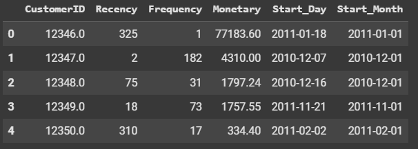
Next, we will examine outliers in our data. Outliers are unusual values in our dataset, and they can distort statistical analyses and violate their assumption. We will first look at the outliers and decide what to do with it.
#Plot RFM outliers
sns.boxplot(x = RFM_df["Recency"])
sns.boxplot(x = RFM_df["Frequency"])
sns.boxplot(x = RFM_df["Monetary"])
Output for 3 graphs:
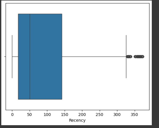
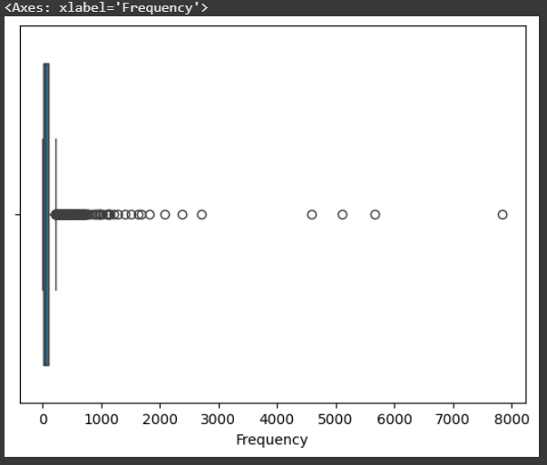
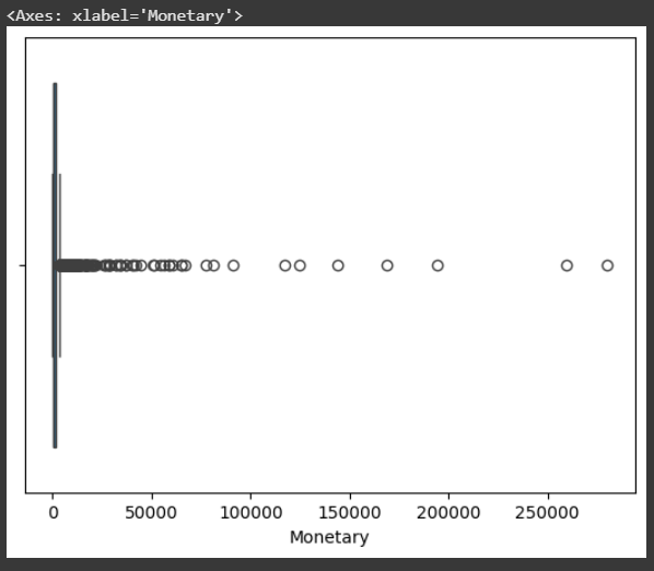
Later, we will have to divide RFM scores into 5 groups using quantile for further analysis. By doing that, we realize that outliers would play a significant role in shifting our data on the wrong scale. Since that would heavily influence our results, we would need to get rid of outliers. I will present 2 ways that we could eliminate outliers
Note: A quantile is a cut point or line of division that splits a probability distribution into continuous intervals with equal probabilities.
# Handle outliers
R_threshold = RFM_df['Recency'].quantile(0.95)
F_threshold = RFM_df['Frequency'].quantile(0.95)
M_threshold = RFM_df['Monetary'].quantile(0.95)

RFM_df_drop_outliers = RFM_df[(RFM_df.Recency <=  R_threshold) & \
                     (RFM_df.Frequency <=  F_threshold) & \
                     (RFM_df.Monetary <=  M_threshold)]

RFM_df_drop_outliers.shape
Output
(3795, 6)
Graphs after drop outliers
# RFM_df_drop_outliers
sns.boxplot(x = RFM_df_drop_outliers["Recency"])
sns.boxplot(x = RFM_df_drop_outliers["Frequency"])
sns.boxplot(x = RFM_df_drop_outliers["Monetary"])
Output of 3 graphs after drop outliers:
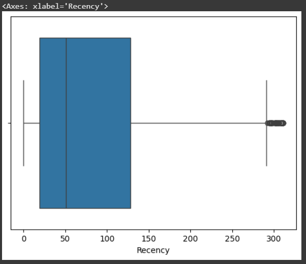
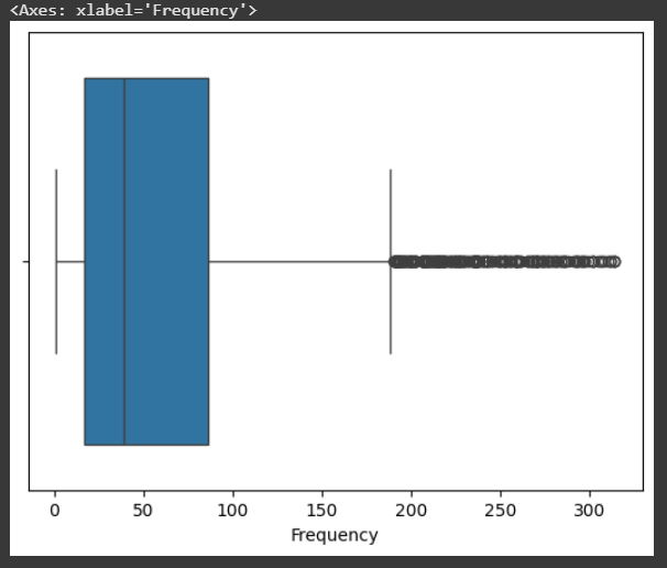
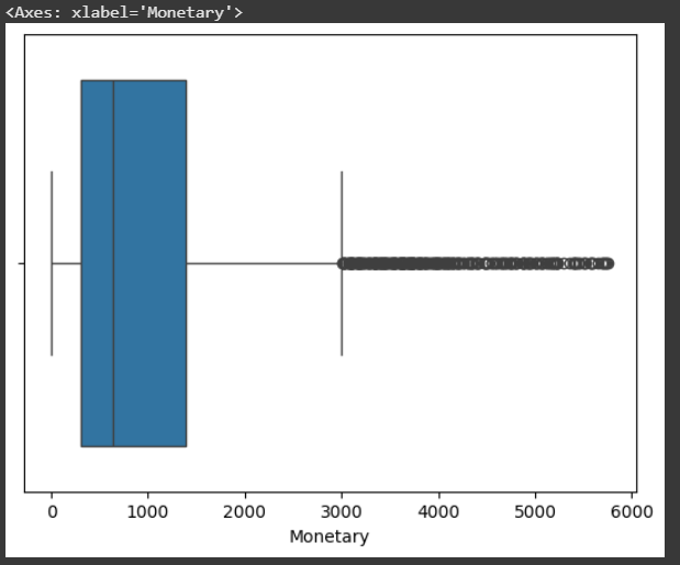
We will continue to map the score from 1-5 for each R, F, M columns
# Using qcut to create R, F, M
RFM_df['R'] = pd.qcut(RFM_df["Recency"], 5, labels = range(1, 6)).astype(str)
RFM_df['F'] = pd.qcut(RFM_df["Frequency"], 5, labels = range(1, 6)).astype(str)
RFM_df['M'] = pd.qcut(RFM_df["Monetary"], 5, labels = range(1, 6)).astype(str)
RFM_df['RFM'] = RFM_df.apply(lambda x: x.R + x.F + x.M, axis = 1)
RFM_df.head()
Output:

Next step, we will import a segmentation file to merge each segment to equivalent RFM score
# Import segmentation file
seg = pd.read_excel(path + 'ecommerce retail.xlsx', sheet_name = 'Segmentation')
seg['RFM Score'] = seg['RFM Score'].str.split(',')
seg = seg.explode('RFM Score').reset_index(drop = True)

# Merge proper Segmentation
RFM_df_final = RFM_df.merge(seg, how = 'left', left_on = 'RFM', right_on = 'RFM Score')
RFM_df_final.head()
Output:

There might be some extra space in RFM Score column when we import it from Excel, which might prevent tables from mapping correctly. We will need to clean up that extra space.
# remove space of Column "RFM Score"
seg['RFM Score'] = seg['RFM Score'].apply(lambda x: x.replace(" ", ""))

#Merge again after removing extra space
RFM_df_final = RFM_df.merge(seg, how = 'left', left_on = 'RFM', right_on = 'RFM Score')
RFM_df_final.head()
Output:

Visualization RFM Model
We would like to understand the distribution of users to define which group/segment has contributed significantly to SuperStore. From there, the marketing team could customize a promotion plan for each group.
# Distribution using Customer Frequency and Monetary
segment_by_user_count = RFM_df_final[['Segment','CustomerID']].groupby(['Segment']).count().reset_index().rename(columns = {'CustomerID':'user_volume'})
segment_by_user_count['contribution_percent'] = round(segment_by_user_count['user_volume'] / segment_by_user_count['user_volume'].sum() * 100)
segment_by_user_count['type'] = 'user contribution'

segment_by_spending = RFM_df_final[['Segment','Monetary']].groupby(['Segment']).sum().reset_index().rename(columns = {'Monetary':'spending'})
segment_by_spending['contribution_percent'] = segment_by_spending['spending'] / segment_by_spending['spending'].sum() * 100
segment_by_spending['type'] = 'spending contribution'

segment_agg = pd.concat([segment_by_user_count, segment_by_spending])

# Set the figure size
plt.figure(figsize=(15, 8))
sns.barplot(segment_agg, x="Segment", y="contribution_percent", hue="type")
plt.title('The overal distribution of User Profile using RFM Model')

# Show the plot
plt.show()
Output:
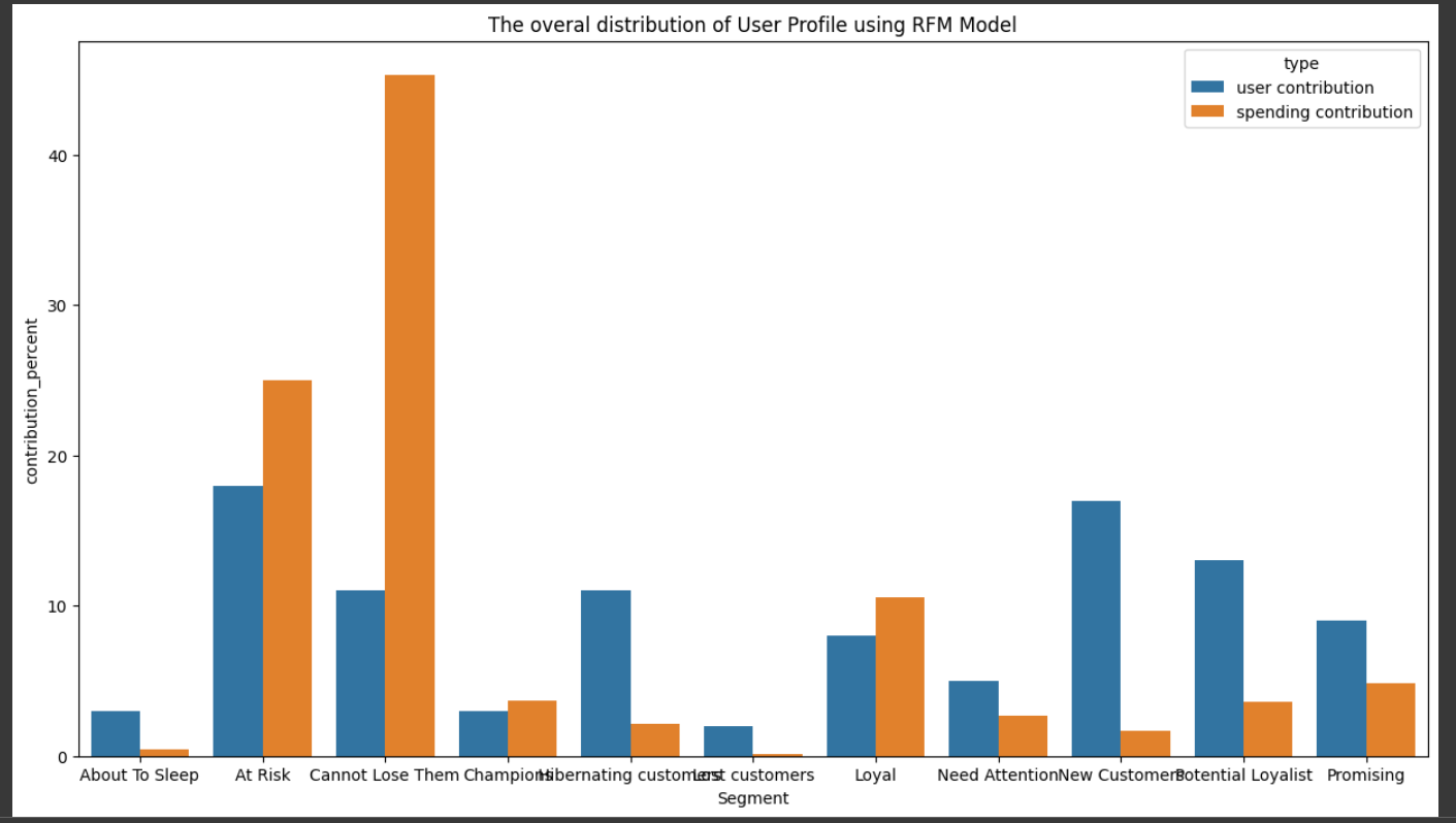
The At Risk and Cannot Lose Them customer segments are critical, as they represent a significant portion of the customer base and contribute substantially to revenue. However, the high proportion of these segments is a warning sign, indicating that many customers have not engaged with the product for a long time and are at high risk of churn.
Recommended Actions: Implement targeted promotional campaigns or personalized notifications to re-engage these customers and encourage product usage.
On the other hand, the Loyal, New Customer, Potential Loyalist, and Promising segments also make up a large portion of the customer base. However, most of these customers have relatively low transaction values and contribute only modestly to overall revenue.
Recommended Actions: Strengthen cross-selling initiatives and promotional strategies to drive higher consumption and increase customer lifetime value.
RFM Distribution throughout the time
We continue to pivot and group user by customer volume & spending by each month.
RFM Customer Volume Distribution by Month
# Process data to visualize stacked column chart with Ox = month, Oy = User volume, Stacked = Segment
RFM_df_final_aggregate_month = RFM_df_final[['Start_Month','Segment','CustomerID','Monetary']]\
                                           .groupby(['Start_Month','Segment']).agg({'CustomerID' : 'count', 'Monetary' : 'sum'}).reset_index().rename(columns = {'CustomerID' : 'Customer_Volume'})

RFM_df_final_aggregate_month['Start_Month'] = RFM_df_final_aggregate_month['Start_Month'].dt.date

RFM_df_final_aggregate_month_pivot_customer = pd.pivot_table(RFM_df_final_aggregate_month, values='Customer_Volume', index = ['Start_Month'], columns = ['Segment']).reset_index()
RFM_df_final_aggregate_month_pivot_customer.index = RFM_df_final_aggregate_month_pivot_customer.Start_Month
RFM_df_final_aggregate_month_pivot_customer = RFM_df_final_aggregate_month_pivot_customer.fillna(0).drop(columns = 'Start_Month')

Custom_colors = ['#845ec2', '#ffc75f', '#d65db1', '#f9f871', '#ff6f91', '#2c73d2', '#ff9671', '#008e9b', '#008f7a', '#b39cd0', '#fbeaff']
ax = RFM_df_final_aggregate_month_pivot_customer.plot(kind='bar', stacked=True)

plt.xticks(rotation=90)  # Rotate x-axis labels for better readability
plt.tight_layout() # Adjust layout to prevent overlapping
ax.legend(bbox_to_anchor=(1.05, 1), loc='upper left', fontsize='small', ncol=2)
plt.title('User Distribution by Segmentation & User Enter Month')
plt.show()
Output:
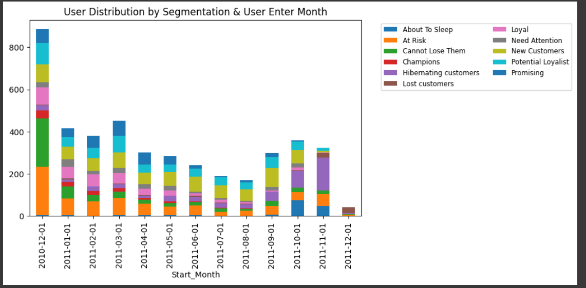
In recent months (September, October, November), the number of Hibernating customers has increased significantly. This is a negative signal, as Hibernating customers typically exhibit poor performance across all three RFM metrics.
Recommended Actions: Further investigate the root causes by analyzing user profiles (e.g., demographics) compared to the general user base to identify any distinctive characteristics. Based on these insights, develop strategies to attract high-value customers while filtering out low-value segments.
The declining customer trend over the past months is also a concerning sign.
Recommended Actions: Implement strategies to sustain a stable customer base over time and prevent further decline.
RFM Customer Spending Distribution by Month
RFM_df_final_aggregate_month_pivot_spending = pd.pivot_table(RFM_df_final_aggregate_month, values='Monetary', index = ['Start_Month'], columns = ['Segment']).reset_index()
RFM_df_final_aggregate_month_pivot_spending.index = RFM_df_final_aggregate_month_pivot_spending.Start_Month
RFM_df_final_aggregate_month_pivot_spending = RFM_df_final_aggregate_month_pivot_spending.fillna(0).drop(columns = 'Start_Month')

Custom_colors = ['#845ec2', '#ffc75f', '#d65db1', '#f9f871', '#ff6f91', '#2c73d2', '#ff9671', '#008e9b', '#008f7a', '#b39cd0', '#fbeaff']
ax = RFM_df_final_aggregate_month_pivot_spending.plot(kind='bar', stacked=True)

plt.xticks(rotation=90)  # Rotate x-axis labels for better readability
plt.tight_layout() # Adjust layout to prevent overlapping
ax.legend(bbox_to_anchor=(1.05, 1), loc='upper left', fontsize='small', ncol=2)
plt.title('Spending Distribution by Segmentation & User Enter Month')
plt.show()
Output:
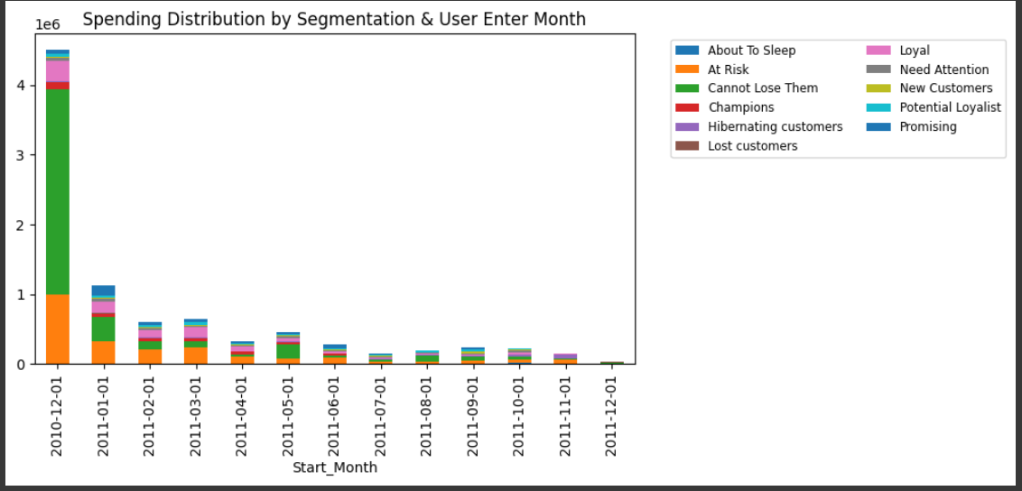
The majority of spending comes from customers who joined the product in December 2010, which is a highly concerning signal.
Recommended Actions: Develop long-term strategies to attract and retain new customers, ensuring a more sustainable revenue stream.
Discussion
To sum up, The At Risk and Cannot Lose Them customer segments play a vital role, as they account for a large share of the customer base and significantly impact revenue. The Loyal, New Customer, Potential Loyalist, and Promising segments constitute a significant share of the customer base. However, the majority of these customers have low spending levels and make a limited contribution to overall revenue. In the last quarter, the number of Hibernating customers has risen sharply, which is a concerning trend. These customers generally perform poorly across all three RFM metrics, indicating low engagement and spending. As well as customer spending has decreased since December 2010.
Action:
- Provide a long-term plan to attract customers and increase customer spending habits
- Come up with a promotion plan for At Risk and Cannot Lose Them customer segments.
- Cross selling & develop new products that potentially interest the Loyal, New Customer, Potential Loyalist, and Promising segments